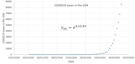
The COVID19 coronavirus pandemic took the world by surprise, and spread unexpectedly. Many countries took emergency measures such as closing their borders, declaring quarantines or curfews.
 |
| Figure 1. COVID19 cases in the USA |
There is much uncertainty as to how cases will increase, and whether or not such measures are reasonable.
In this post we will apply differential equations to explain the spread of the virus and the importance of controlling the risk of infection.
The coronavirus COVID 19 outbreak differential equation
Let's assume y (t) = cases of coronavirus at time t. It shows that "y" is a function of time "t".y (t + Dt) = future coronavirus cases at time t + Dt.
The basis of mathematical epidemiology tells us that the spread of infectious diseases is proportional to the risk of infection R and the time elapsed Dt.
y (t + Dt) = y (t) + y (t) R Dt
Rearranging we have:
[Y (t + Dt) - y (t)] / Dt = R y (t)
Analyzing when Dt is small; that is, when "t" tends to zero (0), we see that the term on the left recalls the mathematical concept of limits, which is equal to the derivative of the function.
Limit [Y (t + Dt) - y (t)] / Dt = dy / dt ; When Dt tends to 0
dy / dt = R y
Which shows us that we have a simple differential equation, which can be solved by separating variables.
dy / y = R dt
Integrating we have:
Ln (y) = Rt + c1
By property of logarithms we have:
y (t) = exp (Rt) * exp (c1)
y (t) = C exp (Rt)
Our initial condition is the so-called patient 0; the first contagion when time is 0, that is, y (0) = 1.
y (0) = C exp (R * 0)
C = 1
Thus, the coronavirus COVID19 equation is:
y (t) = exp (Rt)
Where R is the risk of infection. The value of R depends on many factors such as:
- Exposure. How exposed we are to contagion. For instance, if we go out to parties or to the beach, we expose ourselves; hence, the risk increases. If we don't wash our hands or we don't wear a mask, we also expose ourselves and the risk increases.
- Vulnerability. Older people and people with a weaker immune system are more vulnerable and at higher risk.
In this post we will not go much into the theoretical detail of risk, but we will use a simple empirical approach. From the equation we have:
R = ln (y) / t
Since we have daily data on the number of infected people per day (source: CDC), we can plot the daily risk R variation. Figure 2 shows that risk R is still highly variable. It tends to a value between 0.10 and 0.15. We will assume a risk R of 0.15. Thus, the equation will be:
y (t) = exp (0.15 t)
 |
| Figure 2. COVID19 risk of infection in the USA |
The importance of controlling the risk of infection R
To see the importance of reducing the risk of infection, we will perform a simple sensitivity test considering 3 scenarios:- Scenario in which the risk decreases to 0.14.
- Scenario in which the risk remains constant at 0.15.
- Scenario in which the risk increases to 0.16.
- Risk 0.14: 73 130 cases
- Risk 0.15: 162 754 cases
- Risk 0.16: 362 218 cases
This simple mathematical exercise illustrates the importance of controlling and reducing the risk. Small measures (such as quarantine or washing hands) that would change the risk by 0.01 can make the difference between 73 130 cases and 362 218 cases.
Note 1. It is important to note that the risk R is not constant. This equation is not a universal one. The main objective of this post was to illustrate the importance of reducing the risk by following simple actions such as avoiding crowded areas, quarantine if the government asks you to do it, more control at the borders, washing our hands and many more.
Note 2. The exponential growing corresponds to the first stage of the outbreak. The outbreak does grow exponentially to the infinite. After some time, the trend changes to a Gaussian curve, but that will be covered in another post.
Wow, The post was really nice and amazing to read. Please write a post on the best gift ideas for 2021. I am looking forward. Thanks!
ReplyDeletehttps://giftoper.com/